Making a grid

I'm happy with this blog, I received my first comment (here) this week, thank you Naza Sundae.

Following with our online Scilab's tutorial, let's learn how to make grids, like the figure:

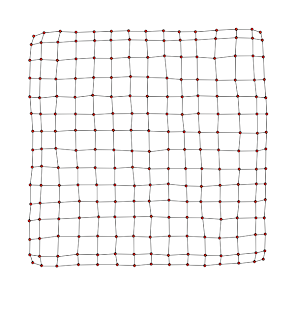
This type of graphs are very important for data visualization.

The first step is to define each point.
Look the example:

(1, 5) - (2, 5) - (3, 5) - (4, 5) - (5, 5)

(1, 4) - (2, 4) - (3, 4) - (4, 4) - (5, 4)

(1, 3) - (2, 3) - (3, 3) - (4, 3) - (5, 3)

(1, 2) - (2, 2) - (3, 2) - (4, 2) - (5, 2)

(1, 1) - (2, 1) - (3, 1) - (4, 1) - (5, 1)

The x-coordinates are the matrix:

X = [1, 2, 3, 4, 5;
1, 2, 3, 4, 5;
1, 2, 3, 4, 5;
1, 2, 3, 4, 5;
1, 2, 3, 4, 5]

And the y-coordinates are the matrix:

Y = [5, 5, 5, 5, 5;
4, 4, 4, 4, 4;
3, 3, 3, 3, 3;
2, 2, 2, 2, 2;
1, 1, 1, 1, 1]

So, we can use the meshgrid function, like presented in the following script:

-->x = meshgrid(1:5)
x =

1. 2. 3. 4. 5.
1. 2. 3. 4. 5.
1. 2. 3. 4. 5.
1. 2. 3. 4. 5.
1. 2. 3. 4. 5.

-->y = meshgrid(5:-1:1)'
y =

5. 5. 5. 5. 5.
4. 4. 4. 4. 4.
3. 3. 3. 3. 3.
2. 2. 2. 2. 2.
1. 1. 1. 1. 1.

-->plot(x, y, 'k.-');

-->plot(x', y', 'k.-');

The result:


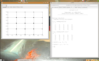
Now, I think it's interesting to upgrade our example.
Look the script:

-->t = 1:20;

-->x = meshgrid(t);

-->y = meshgrid(t($:-1:1))';

-->w = %pi/5;

-->s = sin(w*x);

-->plot(x, s + y, 'b.-');

-->plot(x', (s + y)', 'b.-');

The result:


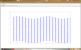
Try to change the grid and look what happens.

Simple graphs - 6

This is the last post about the simple uses of the plot(.) function.

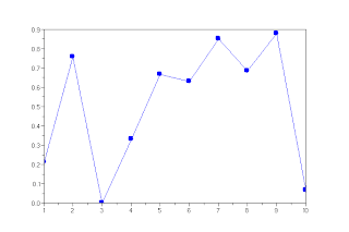
In this post, we will learn how to mark the points on the line's graphs, like the following figure.
The possible styles of markers in Scilab are:

• Plus sign;
• Circle;
• Asterisk;
• Point;
• Cross;
• Square;
• Diamond;
• Upward-pointing triangle;
• Downward-pointing triangle;
• Rightward-pointing triangle;
• Leftward-pointing triangle;
• Five-pointed star (pentagram);
• No marker (default).
  

Those markers may be used with the line's styles (last post) and the colors (before the last post).

Let's do some examples:

-->x1 = rand(10, 1);

-->plot(x1, 'x');

-->plot(x1, 'o');

-->t = 1:10;

-->x2 = exp(-0.1*t);

-->scf(); plot(t, x2, 'sr--');

-->scf(); plot(x1, x2, '^-.g');

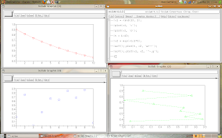
The result:


Ok, now we are ready for start real applications.

Simple graphs - 5

Following our studies about the plot(.) function.

Now, let's learn how to change the line's style.

The possible line's styles in Scilab are:

• Solid line (default);
• Dashed line;
• Dotted line;
• Dash-dotted line;
• No line.
  

Each style may be used with the argument color (cited on the last post).

Some examples:

-->x = 1:10;

-->y1 = x.^2 + 1;

-->plot(x, y1, "-");

-->y2 = x.^2 + 2;

-->plot(x + 10, y2, "--");

-->y3 = x.^2 + 3;

-->plot(x + 20, y3, ":");

-->y4 = x.^2 + 4;

-->plot(x + 30, y4, "-.");


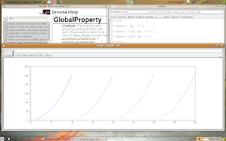
The result:

You may use the line's styles with colors, for example:

--> plot(x, y, "r--");