The convolution is a operation with two functions defined as:

The function in Scilab that implements the convolution is convol(.).
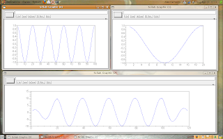
Let's do the test: I'll convolve a cosine (five periods) with itself (one period):
N1 = 100;
N2 = 20;
n1 = 1:N1;
n2 = 1:N2;
w = %pi/10;
f1 = cos(w*n1);
f2 = cos(w*n2);
y = convol(f1, f2);
plot(f1);
scf(); plot(f2);
scf(); plot(y);
The result is:

The top left graph is f1, the top right is f2 and the bottom graph is y.
Again, if anyone wants, I can write about discrete convolution properties.
2 comments:
Yes, i am want it ;p
Discrete Convolution rawks ~~
Hello
You seem to be quite good using Scilab. If you have a few minutes, i'd like to ask you some questions about the convolution via Fourier transform.
Thank you!
Post a Comment