In this post, I want to teach something about basic statistic.
I recommend the Papoulis' book for who intends to study statistic.
Here, I'd like to write about random variables and some operations.
A random variable is a variable that you don't know it value.
In Scilab, random variables are created by the rand(.) function.
The default distribution of probability used in the rand(.) function is uniform (between [0, 1]), but the function supports the normal distribution (with null mean and unitary variance) too.
An example:
x1 = rand()
x1 =
0.5608486
x2 = rand(1, 1, 'uniform') // one line and one column (a scalar variable)
x2 =
0.6623569
x3 = rand(1, 1, 'normal')
x3 =
0.6380837
If you have many values in a variable, like this:
x = rand(10, 1); // ten lines and one column
x =
0.3616361
0.2922267
0.5664249
0.4826472
0.3321719
0.5935095
0.5015342
0.4368588
0.2693125
0.6325745
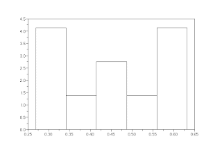
then you can see the histogram using the histplot(.) function.
histplot(5, x); // the function takes the biggest and the smallest values, divides the interval in five parts (the number 5, first argument), and counts how many numbers are in each part
Look the result:

Now, let's do a smarter example:
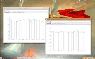
x = rand(10000, 1);
y = 10*x + 2;
histplot(20, x);
scf(); histplot(20, y);
Look the result:

The graphs look like the same, but if you click over the image then you can see the indexes.
The left graph (variable x) has the indexes in the interval [0, 1] and the right graph (variable y) has the indexes in the interval [2, 12].
I ask to my readers: why the indexes are these?
5 comments:
i want a code for gabor filter for texture analysis..pls send me suggestions and code if possible..thanx in advance..
Hi Sivaprasad, I don't know the Gabor filter, but in a fast search I found this code:
function [gb] = gabor_fn(sigma, theta, lambda, psi, gamma)
sigma_x = sigma;
sigma_y = sigma/gamma;
// Bounding box
nstds = 3;
xmax = max(abs(nstds*sigma_x*cos(theta)), abs(nstds*sigma_y*sin(theta)));
xmax = ceil(max(1, xmax));
ymax = max(abs(nstds*sigma_x*sin(theta)), abs(nstds*sigma_y*cos(theta)));
ymax = ceil(max(1, ymax));
xmin = -xmax;
ymin = -ymax;
[x, y] = meshgrid(xmin:xmax, ymin:ymax);
// Rotation
x_theta = x*cos(theta) + y*sin(theta);
y_theta = -x*sin(theta) + y*cos(theta);
gb = exp(-0.5*(x_theta.^2/sigma_x^2 + y_theta.^2/sigma_y^2)).*cos(2*pi/lambda*x_theta + psi);
endfunction
If anyone wants help about subjects that I don't write something yet, I ask: send me an e-mail just for organization in the blog.
Thanks for the compression comprehension.
Hi,
I have two arrays with the following code:
x=[0 0.1 0.2 0.3 0.4 0.5 0.6 0.7 0.8 0.9 1.0];
y=[0.5555556 0.5333333 0.3555556 0.3555556 0.5333333];
histplot(x,y);
When I plot the histplot, it shows a histogram of value 4 between 0.3 - 0.4 and a histogram of value 6 between 0.5 - 0.6. What I want is histogram to count values between 0.3 - 0.4 and show it. The value should be 2 not 4. Also, value for histogram between 0.5 - 0.6 should be 3 not 6.
In short, the histogram is showing twice values on y-axis. How could I fix it?
Thanks.
Probably Scilab is making the histogram with rates instead of counting.
Look for a pattern, changing the values of y.
if you want to count how many samples of y are between 0.3 and 0.4, you could do this:
count = length(find([y > 0.3].*[y < 0.4]));
Regards.
Post a Comment