Simple graphs - 4

Let's continue our study about the plot(.) function.

Now, how change the graph's color?

The plot(.) has a argument that's a string.

We can do:

• plot(x, y, color);
• plot(y, color);
  

Remember, when the x vector isn't in the function, the default is [1:length(y)], where length(y) is the number of elements that y vector has.

The possible colors are:

• red ("r");
• green ("g");
  
• blue ("b");
  
• cyan ("c");
  
• magenta ("m");
  
• yellow ("y");
  
• black ("k");
  
• white ("w").
  

Let's do an example:

-->x = [-100:100]';

-->y1 = abs(x.^3)/1e+5;

-->y2 = x.^3 + x.^2 + 1;

-->y3 = tanh(0.01*x);

-->y2 = y2/max(y2);

-->plot(x, y1);

-->plot(x, y2, "r");

-->plot(x, y3, "g");

-->scf(); plot(x, y2, "k"); plot(x, y3, "y");


This example uses some functions that I had written about, so review the blog if you don't understand anything, or comment here.

The result is following.


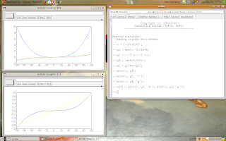
Look that the default color is blue.

Simple graphs - 3

I ask excuse me because I was doing other things, like a paper, and I could not post since 4, April.

Now, I finished the paper, and other things.

Let's continue talking about the plot(.) function.

The command for create a new window is scf(), it creates a blank window.
If you have a used window but you want to clear it, so you use the command clf();

Those commands (scf() and clf()) have no arguments.

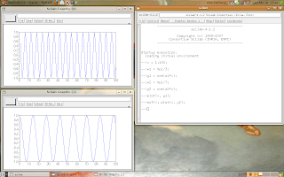
The scf() is utile for show many graphs simultaneously, like the following example.

The script is following, too:

-->x = 1:100;

-->w1 = %pi/3;

-->y1 = cos(w1*x);

-->w2 = %pi/7;

-->y2 = cos(w2*x);

-->plot(x, y1);

-->scf(); plot(x, y2);



The next posts will present how to change the colors and styles of the graphs, and how to put labels on the graphs.

Simple graphs - 2

In the last post I introduced the plot(.) function.

That function is the simplest one for create graphs.

Let's learn something more about that function.

Try the commands:

-->x = rand(10, 1)
x =

0.2113249
0.7560439
0.0002211
0.3303271
0.6653811
0.6283918
0.8497452
0.6857310
0.8782165
0.0683740

-->plot(x);

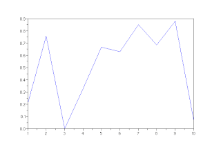
The result is the following picture.

Look the indexes (x axis), it starts on 1 and finishes on 10, because we did not put the x axis in the plot(.).

An other case:

-->y = rand(10, 1)
y =

0.3076091
0.9329616
0.2146008
0.312642
0.3616361
0.2922267
0.5664249
0.4826472
0.3321719
0.5935095

-->x = [0 1 2 3 4 5 6 7 8 9]'
x =

0.
1.
2.
3.
4.
5.
6.
7.
8.
9.

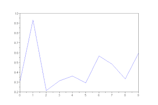
-->plot(x, y);


Now, the x axis starts on 0 and finishes on 9, because I put the coordinates of x axis.