Queue simulation in Scilab

This post is an answer for Agnes, who commented the last post:

Engineering and Scientific Computing with Scilab - Book

This script is a simple simulation of a queue of packs (or anything else) which there are a source, the queue and a destiny.

I coded this script for simulating and problem where there is a source that sends packs with a specific probability, a queue that receives the source packs and stores them, with a maximum number of stored packs, and a destiny that receives the packs from the queue with another specific probability.

All interested ones can run the code and comment it.

N_packs = 15; //total number of packs

P_send = 0.5; //probability of a pack to be sent

P_process = 0.5; //probability of a pack to be processed

N_queue = 10; //maximum number of elements in the queue

N_sent = 0; //number of packs sent to queue

N_line = 0; //number of packs in the queue

N_processed = 0; //number of packs processed

src = rand(N_packs, 2); //source packs

dst = []; //destiny packs

line = []; //queue

processed = []; //processed packs

while N_processed < N_packs,
    try
        plot(src(:,1) + N_queue + 2, src(:,2), '.g'); 

//plots source packs as green dots
    end;
    
    try
        plot(processed(:,1) + N_queue + 2, processed(:,2), '*k'); 

//plots the queue as line of blue dots
    end;
    
    plot(1:N_queue, zeros(1, N_queue), '.w'); //clears queue dots
    
    try
        plot(line(:,1), line(:,2), '.b'); 

//plots the queue as line of blue dots
    end;
    
    try
        plot(dst(:,1), dst(:,2), '.r'); 

//plots destiny packs as red dots
    end;
    
    if rand() < P_send then 

//sends a pack with P_send probability
        if and([N_line < N_queue N_sent < N_packs]) then 

//verifies the queue is full or all packs have been sent
            N_sent = N_sent + 1;
            
            N_line = N_line + 1;
            
            line(N_line,:) = [N_line 0];
            
            processed(N_sent,:) = src(1,:);
            
            src = src(2:$,:);
        end
    end
    
    if rand() < P_process then 

//processes a pack with P_process probability
        if N_line > 0 then 

//verifies the line has at least one pack
            N_processed = N_processed + 1;
            
            N_line = N_line - 1;
            
            line = line(1:N_line,:);
            
            dst(N_processed,:) = -rand(1, 2);
        end
    end
end

Engineering and Scientific Computing with Scilab - Book

I found this book today: Engineering and Scientific Computing with Scilab and there is a very good reference for Scilab users and engineers in general.

The beginning of the book has an introduction about Scilab software and how to use it. In Part II, the book contains information about a specific Systems and Control Toolbox for Scilab.

Part III presents Applications, and here we can apply all knowledge to create and model real systems for simulation and/or real-time control.

This kind of basis makes the difference in undergraduate studies, because the students can easily see and practice their theoretical concepts and improve their problems solving skills.

Using a simulation environment, students can safely test any system and see what happen in many cases and different situations.

So, everyone knows I'm a strong defender of simulations in engineering and all nature sciences, and a book like that is a great signal other people are investing time and work in the same ideal.

However, we must hold in mind, simulation is only the beginning, but it can cut off many problems, specially in design process.

Scilab as software for engineers

I'm an engineer (of telecommunications) and have used Scilab for several years (since 2005). There are many useful tools for image and signal processing, optimization, linear systems and transformations, and general simulations.

Scilab is a software for numerical simulation supported by Scilab Consortium. This group of companies provides resources and services for users and other companies those intend to migrate to an open and stable software platform.

Beyond formal support, Scilab Consortium is an open environment for doubts and discussions where everyone can help and be helped.

About technical resources, Scilab has two ways for developing and application or simulation: script language (Scinotes) or drag-and-drop interface (Scicos), both are powerful but I believe script language is supported by more external toolboxes.

Scilab external toolboxes are freeware and can be downloaded and installed through ATOMS tool (see next picture, click in the figure to enlarge it).

Some links for posts I have published here about my fields of study:

Matrices: http://usingscilab.blogspot.com.br/search/label/matrix

Scilab functions: http://usingscilab.blogspot.com.br/search/label/functions

Fourier Transform: http://usingscilab.blogspot.com.br/search/label/fft

Signal processing: http://usingscilab.blogspot.com.br/search/label/signal%20processing

Image Processing: http://usingscilab.blogspot.com.br/search/label/image%20processing

Data visualization: http://usingscilab.blogspot.com.br/search/label/plot

Statistics: http://usingscilab.blogspot.com.br/search/label/statistic

Mathematics: http://usingscilab.blogspot.com.br/search/label/math

Plotting contours of surfaces

I know there is very useful to see contours of surfaces, many areas use this kind of resource and Scilab has a very simple way to do that.

For a first example, let's use the surface given by the function z = x² + y², this function is a 3D parable. Run the following code for making this surface's graph.


x = -5:0.1:5;
 y = -5:0.1:5;

[xx yy] = meshgrid(x, y);

z = xx.^2 + yy.^2;

plot3d(x, y, z);


The generated graph is like this.

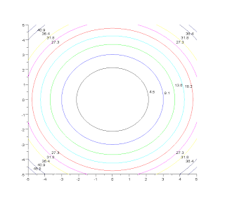
Now, let's see the contours of that surface. But, before, it's interesting to analyze the equation z = x² + y². If z is fixed in a constant value, we have x² + y² = const and this equation means a circle centered in the point (0, 0) and radius square of const.

For plotting the contours, run this code:

n_curves = 10;
x = -5:0.1:5;
y = -5:0.1:5;

function z=my_surface(xx, yy),
z=xx^2 + yy^2;
endfunction

contour(x, y, my_surface, n_curves);


The result is presented following:

In fact, we can see there are concentric circles centered in the point (0, 0).

So, that's all folks!

Plot3d2: creating a cube

For creating a cube with plot3d2(.) function it's required to create three matrices for mapping each vertex of the cube.

Think the six faces of the cube, now open them on a plan and hold each vertex position of the cube. Empty elements of the matrix should be filled according spacial logic of the cube, with the same value of the neighbor vertexes.

-->x = [zeros(4, 2), ones(4, 2), zeros(4, 1)]
 x  =

    0.    0.    1.    1.    0. 
    0.    0.    1.    1.    0. 
    0.    0.    1.    1.    0. 
    0.    0.    1.    1.    0. 

-->y = ones(4, 5);

-->y(2:3,2:3) = 0
 y  =

    1.    1.    1.    1.    1. 
    1.    0.    0.    1.    1. 
    1.    0.    0.    1.    1. 
    1.    1.    1.    1.    1.  

-->z = [zeros(2, 5); ones(2, 5)];
 z  =

    0.    0.    0.    0.    0. 
    0.    0.    0.    0.    0. 
    1.    1.    1.    1.    1. 
    1.    1.    1.    1.    1. 

-->plot3d2(x, y, z);



Result is presented in the following image:

In this case, all faces of the cube are equal, which makes this structure symmetric.

Plot3D: rectangular surface

I received a request of how to create a rectangular surface.

This post is about plot3d(.) function, which I use to create surfaces in Scilab: http://usingscilab.blogspot.com.br/2009/06/plot-3d-surface.html

Now, look plot3d(.) has three arguments: x, y, and z, being the first two ones vectors and the last one is a matrix.

For a surface that x and y are in set [0, 10] and z is in set [0, 1], take the following code:

-->x = 0:10;

-->y = 0:10;

-->z = zeros(length(x), length(y)); // z matrix is initialized with zeros

-->z(($/4):(3*$/4),($/4):(3*$/4)) = 1 // a square in the matrix is set to 1
 z  =

    0.    0.    0.    0.    0.    0.    0.    0.    0.    0.    0. 
    0.    1.    1.    1.    1.    1.    1.    1.    0.    0.    0. 
    0.    1.    1.    1.    1.    1.    1.    1.    0.    0.    0. 
    0.    1.    1.    1.    1.    1.    1.    1.    0.    0.    0. 
    0.    1.    1.    1.    1.    1.    1.    1.    0.    0.    0. 
    0.    1.    1.    1.    1.    1.    1.    1.    0.    0.    0. 
    0.    1.    1.    1.    1.    1.    1.    1.    0.    0.    0. 
    0.    1.    1.    1.    1.    1.    1.    1.    0.    0.    0. 
    0.    0.    0.    0.    0.    0.    0.    0.    0.    0.    0. 
    0.    0.    0.    0.    0.    0.    0.    0.    0.    0.    0. 
    0.    0.    0.    0.    0.    0.    0.    0.    0.    0.    0. 

-->plot3d(x, y, z); // shows the 3d graphic with x, y, and z components



The generated image is the following.

I wish this example has been helpful.

Obs.: for creating a cube, or parallelogram, plot3d2(.) function is more recommended: http://usingscilab.blogspot.com.br/2012/09/plot3d2-creating-cube.html

Gamma function

Last week I was teaching about combinatorial analysis and talking about factorial operator I remembered Gamma Function, this function is very useful in signal processing but particularly Gamma Function is equal to the factorial for non-negative integer numbers.

Theory about Gamma Function is very well described in Wikipedia: http://en.wikipedia.org/wiki/Gamma_function

The equation that defines Gamma Function is

Following figure presents the graph of Gamma Function

And when z is a non-negative integer is verified that

This consequence is because of the property

Typical values of Gamma function are

 In Scilab, there are both functions: gamma(.) and factorial(.), following are some examples of these functions


-->factorial(1)
 ans  =

    1. 

-->gamma(1)
 ans  =

    1. 

-->factorial(1.5)
 !--error 10000
factorial: Wrong value for input argument #1: Scalar/vector/matrix/hypermatrix of positive integers expected.
at line      14 of function factorial called by : 
factorial(1.5)


-->gamma(1.5)
 ans  =

    0.8862269 

-->sqrt(%pi)/2
 ans  =

    0.8862269 

Look factorial(.) is not possible to be applied in a non-integer number, the same happens with negative numbers.

And gamma(.) in 1.5 is equal to sqrt(%pi)/2 verifying the correspondence presented in the typical values figure.


Obs.: all equations and figures that I posted in this text were got from the Wikipedia page.

Scilab Tips

This week I discovered Equalis has a portal for Scilab users shared tips and examples of applications: http://www.equalis.com/blogpost/731635/Scilab-Tips

It's a suggestion for improving Scilab community integration because there are users of everywhere, and if you need anything about Scilab, I believe Equalis portal is the place where you can find anyone that can help you.

Another useful way for using Equalis portal is to make yourself more visible in Scilab community, probably you know something that is the solution for a doubt of other Scilab user.